1 About DynareR

DynareR is an R package that can run Dynare program from R Markdown.

2 Requirements

Users need the following in order to knit this document:

• Dynare 4.6.1 or above

• Octave 5.2.0 or above

3 Installation

DynareR can be installed using the following commands in R.

install.packages("DynareR")

          OR
          
devtools::install_github('sagirumati/DynareR')

4 Usage

Please load the DynareR package as follows:

Then create a chunk for dynare (adopted from Dynare example file BKK) as shown below:

```dynare
/*
 * This file implements the multi-country RBC model with time to build,
 * described in Backus, Kehoe and Kydland (1992): "International Real Business
 * Cycles", Journal of Political Economy, 100(4), 745-775.
 *
 * The notation for the variable names are the same in this file than in the paper.
 * However the timing convention is different: we had to taken into account the
 * fact that in Dynare, if a variable is denoted at the current period, then
 * this variable must be also decided at the current period.
 * Concretely, here are the differences between the paper and the model file:
 * - z_t in the model file is equal to z_{t+1} in the paper
 * - k_t in the model file is equal to k_{t+J} in the paper
 * - s_t in the model file is equal to s_{J,t}=s_{J-1,t+1}=...=s_{1,t+J-1} in the paper
 *
 * The macroprocessor is used in this file to create a loop over countries.
 * Only two countries are used here (as in the paper), but it is easy to add
 * new countries in the corresponding macro-variable and completing the
 * calibration.
 *
 * The calibration is the same than in the paper. The results in terms of
 * moments of variables are very close to that of the paper (but not equal
 * since the authors a different solution method).
 *
 * This implementation was written by Sebastien Villemot. Please note that the
 * following copyright notice only applies to this Dynare implementation of the
 * model.
 */

/*
 * Copyright (C) 2010 Dynare Team
 *
 * This file is part of Dynare.
 *
 * Dynare is free software: you can redistribute it and/or modify
 * it under the terms of the GNU General Public License as published by
 * the Free Software Foundation, either version 3 of the License, or
 * (at your option) any later version.
 *
 * Dynare is distributed in the hope that it will be useful,
 * but WITHOUT ANY WARRANTY; without even the implied warranty of
 * MERCHANTABILITY or FITNESS FOR A PARTICULAR PURPOSE.  See the
 * GNU General Public License for more details.
 *
 * You should have received a copy of the GNU General Public License
 * along with Dynare.  If not, see <http://www.gnu.org/licenses/>.
 */

@#define countries = [ "H", "F" ]
@#define J = 4

@#for co in countries
var C_@{co} L_@{co} N_@{co} A_@{co} K_@{co} Z_@{co} X_@{co} LAMBDA_@{co} S_@{co} NX_@{co} Y_@{co};

varexo E_@{co};

parameters beta_@{co} alpha_@{co} eta_@{co} mu_@{co} gamma_@{co} theta_@{co} nu_@{co} sigma_@{co} delta_@{co} phi_@{co} psi_@{co} rho_@{co}_@{co};
@#endfor

// Lagrange multiplier of aggregate constraint
var LGM;

parameters rho_@{countries[1]}_@{countries[2]} rho_@{countries[2]}_@{countries[1]};

model;
@#for co in countries

Y_@{co} = ((LAMBDA_@{co}*K_@{co}(-@{J})^theta_@{co}*N_@{co}^(1-theta_@{co}))^(-nu_@{co}) + sigma_@{co}*Z_@{co}(-1)^(-nu_@{co}))^(-1/nu_@{co});
K_@{co} = (1-delta_@{co})*K_@{co}(-1) + S_@{co};
X_@{co} =
@# for lag in (-J+1):0
          + phi_@{co}*S_@{co}(@{lag})
@# endfor
;

A_@{co} = (1-eta_@{co})*A_@{co}(-1) + N_@{co};
L_@{co} = 1 - alpha_@{co}*N_@{co} - (1-alpha_@{co})*eta_@{co}*A_@{co}(-1);

// Utility multiplied by gamma
# U_@{co} = (C_@{co}^mu_@{co}*L_@{co}^(1-mu_@{co}))^gamma_@{co};

// FOC with respect to consumption
psi_@{co}*mu_@{co}/C_@{co}*U_@{co} = LGM;

// FOC with respect to labor
// NOTE: this condition is only valid for alpha = 1
psi_@{co}*(1-mu_@{co})/L_@{co}*U_@{co}*(-alpha_@{co}) = - LGM * (1-theta_@{co})/N_@{co}*(LAMBDA_@{co}*K_@{co}(-@{J})^theta_@{co}*N_@{co}^(1-theta_@{co}))^(-nu_@{co})*Y_@{co}^(1+nu_@{co});

// FOC with respect to capital
@# for lag in 0:(J-1)
 +beta_@{co}^@{lag}*LGM(+@{lag})*phi_@{co}
@# endfor
@# for lag in 1:J
 -beta_@{co}^@{lag}*LGM(+@{lag})*phi_@{co}*(1-delta_@{co})
@# endfor
 = beta_@{co}^@{J}*LGM(+@{J})*theta_@{co}/K_@{co}*(LAMBDA_@{co}(+@{J})*K_@{co}^theta_@{co}*N_@{co}(+@{J})^(1-theta_@{co}))^(-nu_@{co})*Y_@{co}(+@{J})^(1+nu_@{co});

// FOC with respect to stock of inventories
 LGM=beta_@{co}*LGM(+1)*(1+sigma_@{co}*Z_@{co}^(-nu_@{co}-1)*Y_@{co}(+1)^(1+nu_@{co}));

// Shock process
@# if co == countries[1]
@#  define alt_co = countries[2]
@# else
@#  define alt_co = countries[1]
@# endif
 (LAMBDA_@{co}-1) = rho_@{co}_@{co}*(LAMBDA_@{co}(-1)-1) + rho_@{co}_@{alt_co}*(LAMBDA_@{alt_co}(-1)-1) + E_@{co};


NX_@{co} = (Y_@{co} - (C_@{co} + X_@{co} + Z_@{co} - Z_@{co}(-1)))/Y_@{co};

@#endfor

// World ressource constraint
@#for co in countries
  +C_@{co} + X_@{co} + Z_@{co} - Z_@{co}(-1)
@#endfor
    =
@#for co in countries
  +Y_@{co}
@#endfor
    ;

end;

@#for co in countries
beta_@{co} = 0.99;
mu_@{co} = 0.34;
gamma_@{co} = -1.0;
alpha_@{co} = 1;
eta_@{co} = 0.5; // Irrelevant when alpha=1
theta_@{co} = 0.36;
nu_@{co} = 3;
sigma_@{co} = 0.01;
delta_@{co} = 0.025;
phi_@{co} = 1/@{J};
psi_@{co} = 0.5;
@#endfor

rho_H_H = 0.906;
rho_F_F = 0.906;
rho_H_F = 0.088;
rho_F_H = 0.088;

initval;
@#for co in countries
LAMBDA_@{co} = 1;
NX_@{co} = 0;
Z_@{co} = 1;
A_@{co} = 1;
L_@{co} = 0.5;
N_@{co} = 0.5;
Y_@{co} = 1;
K_@{co} = 1;
C_@{co} = 1;
S_@{co} = 1;
X_@{co} = 1;

E_@{co} = 0;
@#endfor

LGM = 1;
end;

shocks;
var E_H; stderr 0.00852;
var E_F; stderr 0.00852;
corr E_H, E_F = 0.258;
end;

steady;
check;

stoch_simul(order=1, hp_filter=1600, nograph);
```

The above chunk creates a Dynare program with the chunk’s content, then automatically run Dynare, which will save Dynare outputs in the current directory.

Please note that DynareR uses the chunk name as the model name. So, the outpus of Dynare are saved in a folder with its respective chunk name. Thus a new folder BKK will be created in your current working directory.

5 Plotting the IRF

The Impulse Response Function (IRF) is saved by default in BKK/BKK/graphs/ folder with the IRF’s name BKK_IRF_E_H2.pdf, where BKK is the Dynare model’s name.

5.1 The include_IRF function

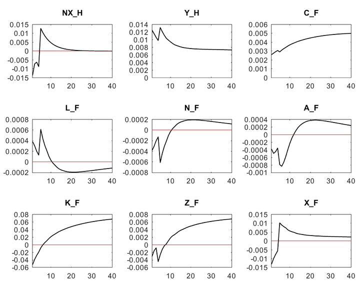
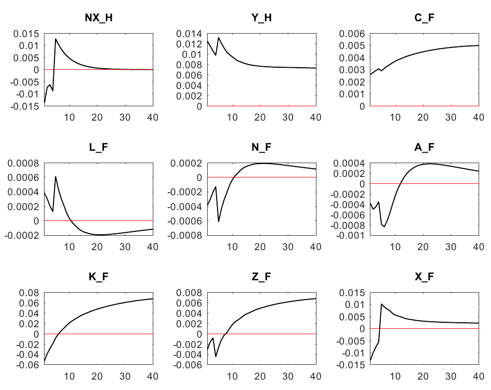
Use this function to embed the graphs of Impulse Response Function (IRF) in R Markdown document.

The Impulse Response Function (IRF) of the BKK model can be fetched using the following R chunk. Note that only the last part of the IRF’s name (E_H2) is needed, that is BKK_IRF_ is excluded. Also note that out.extra='trim={0cm 7cm 0cm 7cm},clip' is used to trim the white space above and below the IRF

```{r IRF,out.extra='trim={0cm 7cm 0cm 7cm},clip',fig.cap="Another of figure generated from Dynare software"}  
include_IRF("BKK","E_H2")
```

Figure 5.1: Example of an IRF imported using include_IRF function

However, Dynare figure can only be dynamically included if the output format is pdf as Dynare produces pdf and eps graphs only.

6 DynareR functions for base R

The DynareR package is also designed to work with base R. The following functions show how to work with DynareR outside R Markdown.

write_dyn(model, code, path = "")

DynareCodes='var y, c, k, a, h, b;
varexo e, u;
parameters beta, rho, alpha, delta, theta, psi, tau;
alpha = 0.36;
rho   = 0.95;
tau   = 0.025;
beta  = 0.99;
delta = 0.025;
psi   = 0;
theta = 2.95;
phi   = 0.1;
model;
c*theta*h^(1+psi)=(1-alpha)*y;
k = beta*(((exp(b)*c)/(exp(b(+1))*c(+1)))
          *(exp(b(+1))*alpha*y(+1)+(1-delta)*k));
y = exp(a)*(k(-1)^alpha)*(h^(1-alpha));
k = exp(b)*(y-c)+(1-delta)*k(-1);
a = rho*a(-1)+tau*b(-1) + e;
b = tau*a(-1)+rho*b(-1) + u;
end;
initval;
y = 1.08068253095672;
c = 0.80359242014163;
h = 0.29175631001732;
k = 11.08360443260358;
a = 0;
b = 0;
e = 0;
u = 0;
end;

shocks;
var e; stderr 0.009;
var u; stderr 0.009;
var e, u = phi*0.009*0.009;
end;

stoch_simul;'

model<-"example1"  
code<-DynareCodes

write_dyn(model,code)

write_mod(model, code, path = "")

DynareCodes='var y, c, k, a, h, b;
varexo e, u;
parameters beta, rho, alpha, delta, theta, psi, tau;
alpha = 0.36;
rho   = 0.95;
tau   = 0.025;
beta  = 0.99;
delta = 0.025;
psi   = 0;
theta = 2.95;
phi   = 0.1;
model;
c*theta*h^(1+psi)=(1-alpha)*y;
k = beta*(((exp(b)*c)/(exp(b(+1))*c(+1)))
          *(exp(b(+1))*alpha*y(+1)+(1-delta)*k));
y = exp(a)*(k(-1)^alpha)*(h^(1-alpha));
k = exp(b)*(y-c)+(1-delta)*k(-1);
a = rho*a(-1)+tau*b(-1) + e;
b = tau*a(-1)+rho*b(-1) + u;
end;
initval;
y = 1.08068253095672;
c = 0.80359242014163;
h = 0.29175631001732;
k = 11.08360443260358;
a = 0;
b = 0;
e = 0;
u = 0;
end;

shocks;
var e; stderr 0.009;
var u; stderr 0.009;
var e, u = phi*0.009*0.009;
end;

stoch_simul;'

model<-"example1"  
code<-DynareCodes

write_mod(model,code)

run_dynare(model,code,path)

DynareCodes='var y, c, k, a, h, b;
varexo e, u;
parameters beta, rho, alpha, delta, theta, psi, tau;
alpha = 0.36;
rho   = 0.95;
tau   = 0.025;
beta  = 0.99;
delta = 0.025;
psi   = 0;
theta = 2.95;
phi   = 0.1;
model;
c*theta*h^(1+psi)=(1-alpha)*y;
k = beta*(((exp(b)*c)/(exp(b(+1))*c(+1)))
          *(exp(b(+1))*alpha*y(+1)+(1-delta)*k));
y = exp(a)*(k(-1)^alpha)*(h^(1-alpha));
k = exp(b)*(y-c)+(1-delta)*k(-1);
a = rho*a(-1)+tau*b(-1) + e;
b = tau*a(-1)+rho*b(-1) + u;
end;
initval;
y = 1.08068253095672;
c = 0.80359242014163;
h = 0.29175631001732;
k = 11.08360443260358;
a = 0;
b = 0;
e = 0;
u = 0;
end;

shocks;
var e; stderr 0.009;
var u; stderr 0.009;
var e, u = phi*0.009*0.009;
end;

stoch_simul;'

model<-"example1"  
code<-DynareCodes

run_dynare(model,code)

run_models(model, path = "")

model=c("example1","example2","agtrend","bkk")
run_models(model)

7 Demo

The demo files are included and can be accessed via demo(package=“DynareR”)

8 Template

Template for R Markdown is created. Go to file->New File->R Markdown-> From Template->DynareR.

9 Examples

The examples folder contains R scripts for demonstrating the use of DynareR. We use “example1” of the Dynare example files for all the functions.

10 STEPS to run the Dynare files

1. Please load the DynareR package in R using the following code

2. Please enusre that the “current working directory” is “examples” folder.

3. Please run the R scripts individually using the following codes:

If you are using R Studio, you can open each of the files above and run the entire codes.

4. Please run all the above models using the following code:

You can also open the run_all.R file in R Studio and run the entire code.

The outputs of each model (example1, bkk, agtrend etc) will be saved in a new folder with the model’s name created in the current working directory (demo). The outputs of each DynareR function (write_mod, write_dyn, run_dynare) will be saved in a folder with the function’s name.

11 Working existing mod files

The folder DynareFiles contains the Dynare built-in example files

12 STEPS to run the Dynare built-in example files

1. If DynareR package is not installed on your R, please install it using the following codes

2. Please load the DynareR package in R using the following code

3. Please enusre that the “current working directory” is DynareFiles folder.

4. Please run a single model using the following code:

5. Please run multiple models using the following code

7. If the files live in different folder from the R “current working directory”, please provide the folder,for example, as follows:

Then use the following codes to run the models:

To run a single Dynare model;

To run multiple existing Dynare models;

The outputs of each model (example1, bkk, agtrend etc) will be saved in a new folder with the model’s name created in the current working directory (DynareFiles).

Please visit my Github for a better explanation and example files.